


How to read spectrographs and tables correctly
In our tests, you will increasingly encounter measurements of the “frequency response” of the sound of PC components. These are useful and rare measurements. As one of our readers has pointed out – for those who can read spectrographs, they are a gem. It’s worse if you don’t understand them. Then they won’t tell you much, and that’s a shame if you also care about the exact “noise” value of computer components, or their sound expression.
How to read spectrographs and tables correctly
Longtime readers know well why we began to measure the frequency response of the sound of PC components. However, this term may also be of interest to those of you who have not yet encountered it (you basically didn’t have a chance to in hardware tests…), but you still care about the sound the computer makes. It will matter to the vast majority, I dare say. After all, no one likes computers whose noise level reaches the level of vacuum cleaners, but also those where you, on the one hand, don’t measure high decibels on the sound level meter, but at the same time your ears are burning. This typically includes whistling, whirring and similar irritating noises.
The easiest way to analyze noise is to use a sound level meter. We also use it, but it has several limitations from the principle of its functioning. First of all, the disadvantage is that the sound level meter senses the noise level across an entire frequency bandwidth and gives you a value of “sound pressure” at the output. This quantity indicates whether, under certain conditions of use (measured device/sound level meter), the object of interest is noisy, quiet or something in between. But it will not give you a clear idea of how the sound of the measured device sounds. That is, unless you currently have an extremely expensive sound level meter with its own spectrograph. But even these usually have a resolution of only 1/3 octave, i.e. lower than the one we work with. In any case, a standard sound level meter, which has only one value (dBa/dBc) at the output, evaluates it based on a mix of all frequencies, and the result says nothing about whether it is 40 dBA booming or squeaky. And this is a fundamental difference from the user’s point of view.
Imagine choosing the quietest in a test of thirty graphics cards, because its measured noise level is only “30.1 dBA” (that is, at the limit of what ordinary sound level meters can record), but in the end you find your old “32-decibel” card’s noise a bit more pleasant. This can easily happen, because the new card may have dominant frequencies that do not suit you. Therefore, in addition to taking into account the total noise level, it is appropriate to analyze which frequencies are more and which are less dominant in the overall sound of a particular cooler or graphics card as a whole (because non-cooling elements, typically coils, contribute to the results as well).
The human ear perceives sound frequencies in the range of approximately 20–20,000 Hz. Of course, everyone is different and it changes with age, too. But the reference scale is optimal and that is why we also measure in this range. Notice the horizontal axis in the graph below where 20 Hz is on the left and 20,000 Hz on the far right. You will know the difference between low and high frequencies and some more detailed descriptions and comparisons will not be necessary. In short, the higher the frequencies, the more squeaky the sound and vice versa (low frequencies, bass, are relatively dull). From 20 Hz to 20 kHz, however, the path is relatively long and the individual tones on it need to be distinguished with sufficient subtlety, in small steps. These are determined by fractions of an octave. We mentioned above that some expensive sound level meters have a spectrograph, which has only 1/3 octave, which can fit only 36 samples, or different frequencies that are analyzed. It’s better than nothing, but why impoverish the analysis when you get finer data from 240 samples in the same time unit at 1/24 octave. The highest paid version of TrueRTA also allows such accurate recording of the measured sound.
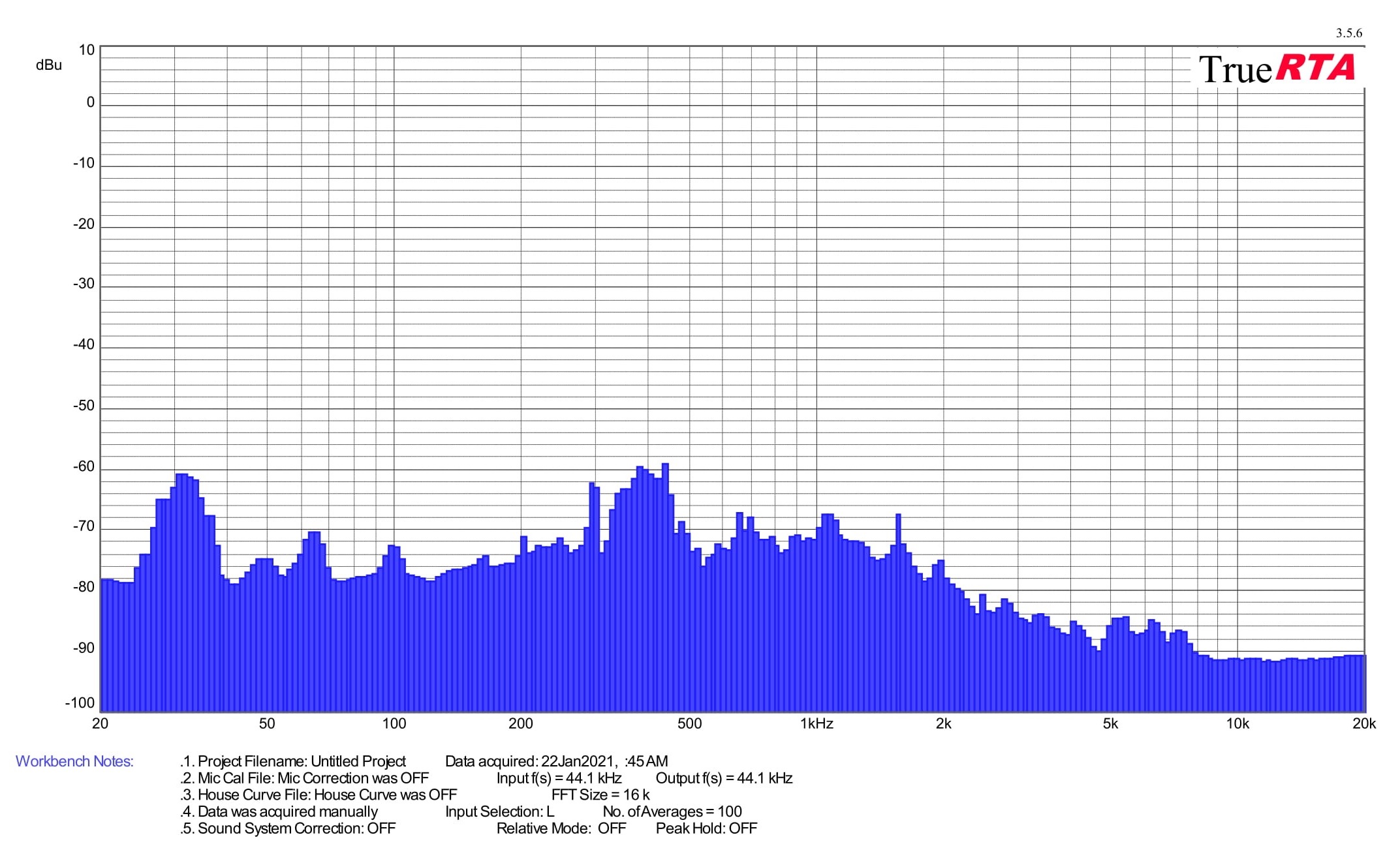
On the vertical axis there is then the intensity of the noise to which the specific frequency extends. That is, which is noisier and which is less. The shape of the spectrograph itself reveals the relative proportions of the frequencies within one measurement, but across multiple measurements (typically when comparing different components), it makes sense to operate with the intensity of the same frequencies. In the original tests, we extracted into the dominant graphs only the dominant frequencies in the three bands of low (20–200 Hz), middle (201–2,000 Hz) and high (2,001–20,000 Hz) tones. However, based on your feedback, we’ve determined and found it appropriate to indicate the intensity of specific frequencies. After all, a particular dominant frequency may be the same for two different sound sources, but one is more ear-piercing than the other.
And one important thing. Don’t be fooled by the dBu weight wide-spread in music. You usually encounter dBa in tests, which we also use when measuring the level with a sound level meter. However, we will stick to dBu for the frequency response of sound. There are several reasons for that. It is possible to convert, and if you need it for some reason, add the value 85 to our measured values and you have it in dBa. However, we will not do it (Miro, I’m sorry. I believe you will get over it…).
Considering that the used TrueRTA application does not natively evaluate the weight of dBa, even after that recalculation, these data could be misleading and someone could compare them with the measured noise levels with which the dBa measured by the miniDSP UMIK-1 microphone would be completely incompatible. On the one hand, we continuously calibrate the sound level meter with a calibrated digital sound level meter Voltcraft SLC-100 certified by a technical testing institute, compared to which the miniDSP UMIK-1 microphone would of course be inaccurate. It also has a calibrated profile, but to a different application (REW) and not TrueRTA. On the one hand, the Reed R8080 has a completely different measuring range for dB (our sound level meter has 30–130 dB) and after calculating the measured values from TrueRTA, you will get values well below 30 dBa. In short, a different metric with the same units, readers who are in a hurry would be offered meaningless comparisons. This is one of the reasons why we prefer raw results in dBu. Last but not least, it saves time when processing the results.
Anyway, these are not absolute numbers, we do not measure according to any standard, but in such a way that the measurements can be compared with each other as best as possible with regard to specific types of components. Mutual differences are important and it does not matter in which units they are interpreted. It is always true that a higher number means higher noise. But with dBu, keep in mind that they are expressed as a negative value. This means that the frequency that is closer to zero has a higher noise intensity. So -70 dBu means higher noise than -75 dBu.
The article continues with the second chapter, which you can go to with the red “Next Chapter” button on the right (or by clicking this link).
In our tests, you will increasingly encounter measurements of the “frequency response” of the sound of PC components. These are useful and rare measurements. As one of our readers has pointed out – for those who can read spectrographs, they are a gem. It’s worse if you don’t understand them. Then they won’t tell you much, and that’s a shame if you also care about the exact “noise” value of computer components, or their sound expression.
Measuring the same value twice in a row is difficult
If you hold your breath while measuring the noise level with a standard sound level meter, you’ll go crazy when measuring the frequency response. It is not at all easy to measure the same values of the same sound repeatedly. Purposely choose a constant sound source and record its frequency response several times during the day. All you need is a regular microphone and one octave, which is available in the free version of TrueRTA (you can download it here).
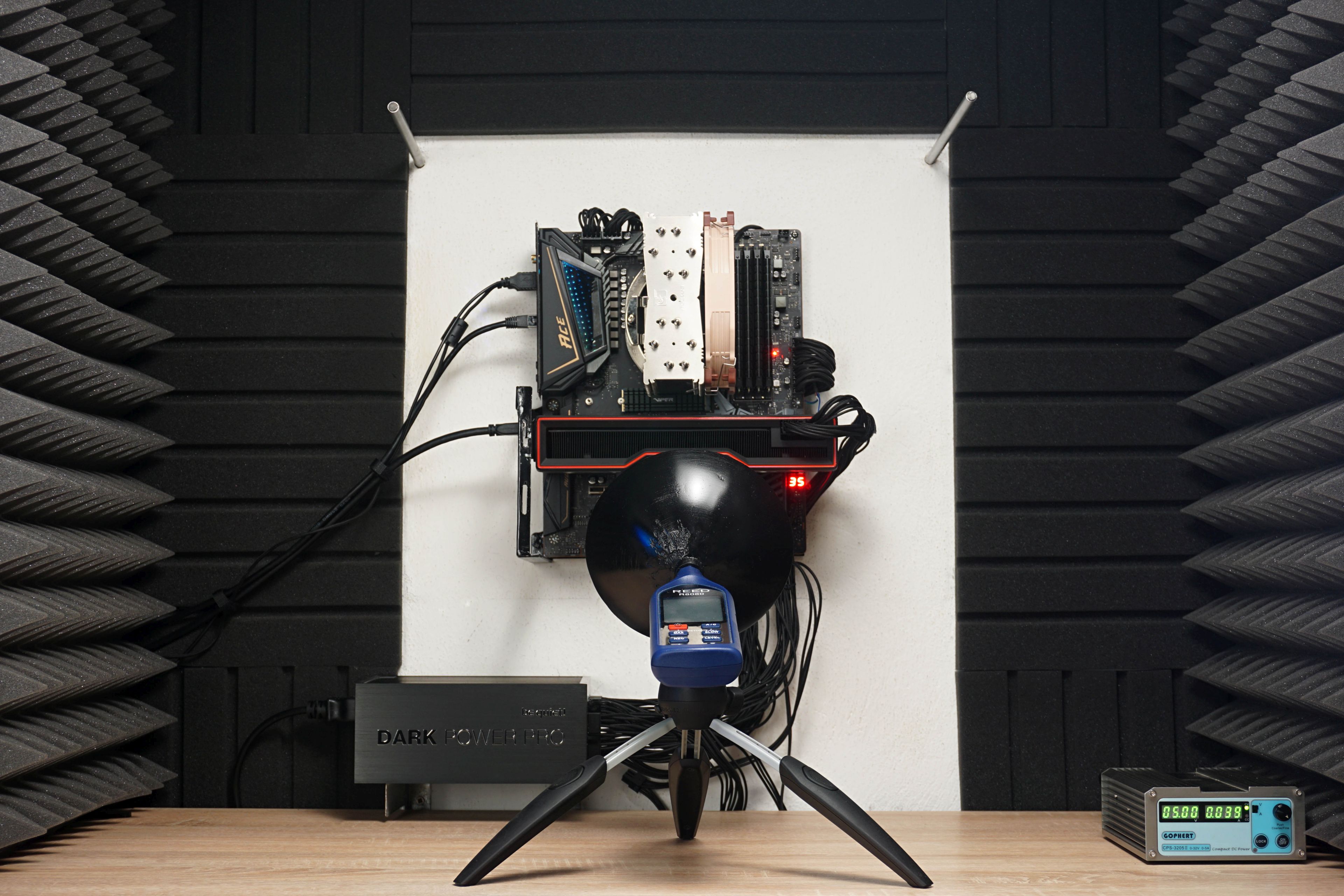
You can’t easily get completely identical graphs across measurements, and we were frustrated by that too. However, with the help of various gimmicks, we reached a very small, negligible measurement error, which fits below 2%. It is important to create completely identical conditions here, in which only the sound of the measured device changes. Around the test rig, we had to place acoustic panels from three sides (from the sides and above), which prevent the sound from bouncing differently into the microphone sensor. Whether the sound from the measured device or from the room. After all, it is quite uncomfortable to commit that nothing will change in the testlab dispositionally just because it would have a negative effect on the accuracy of the measurements.
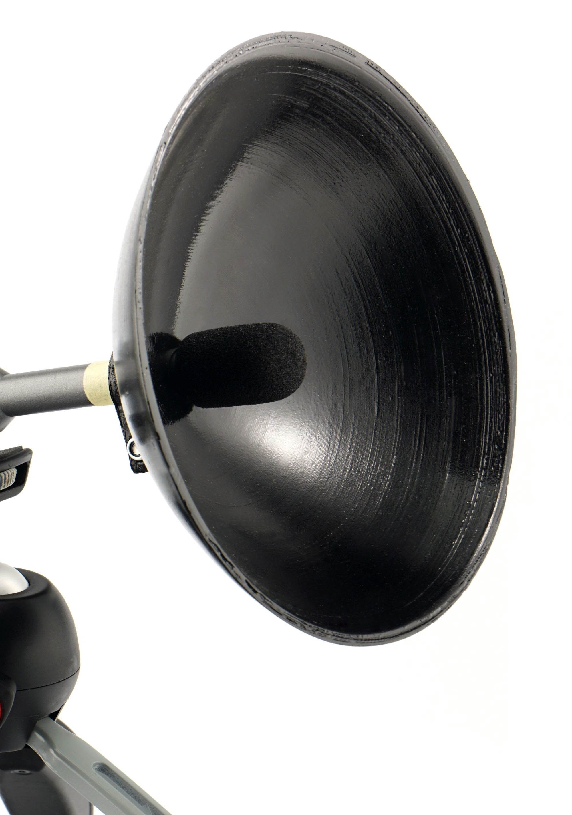
There is then a parabola-shaped collar around the sensor, one of the tasks of which is to amplify the measured values. This makes it possible to distinguish even really quiet frequencies and also so that the spurious tones coming from behind are bounced outside the sensor. Thus, for example, the breathing, which I unfortunately cannot avoid, is possible to filter out in this way.
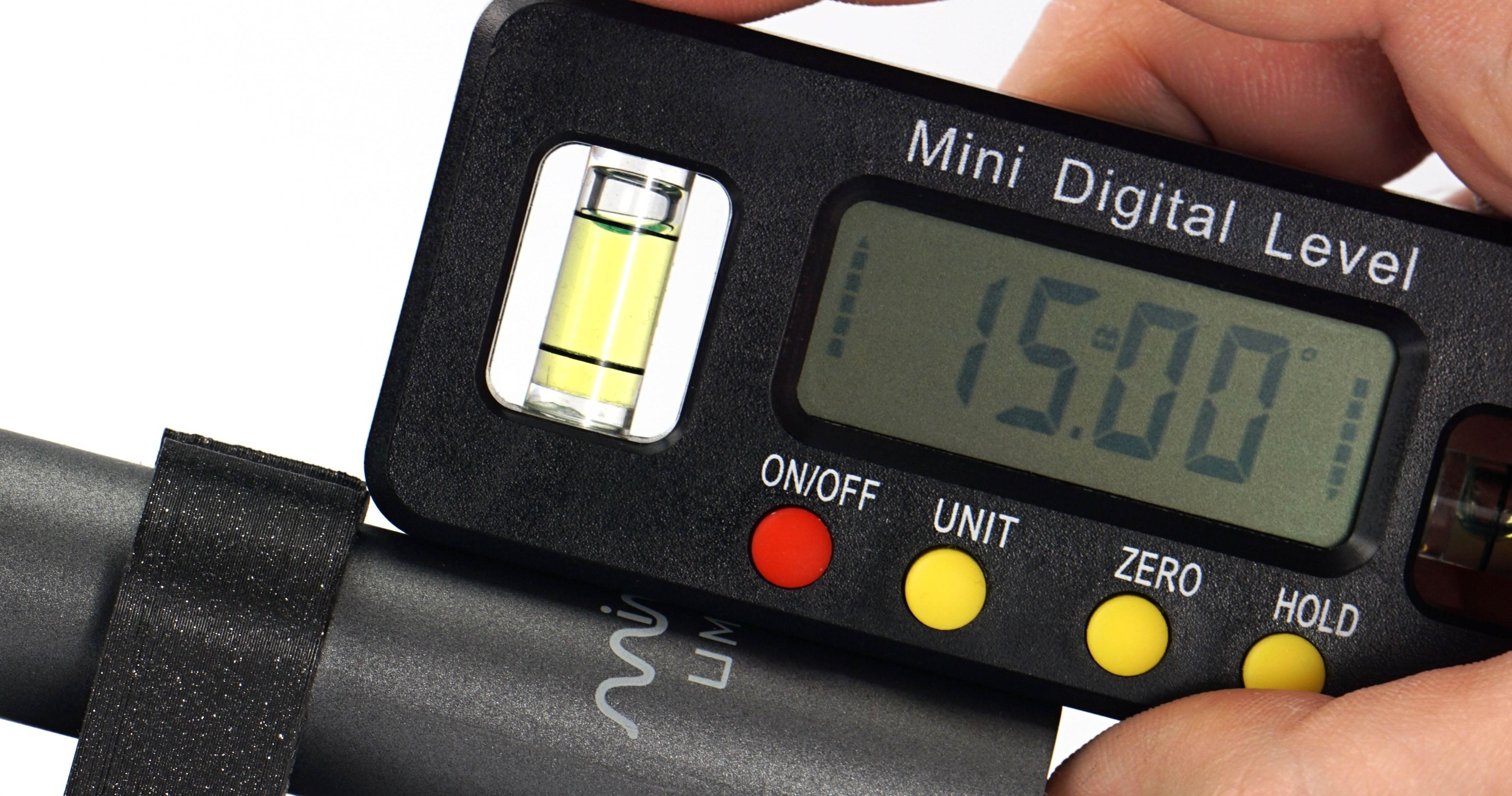
The same mutual distances of the microphone from the measured device, the scanning angle (15°) are always important, too. We always set the angle exactly with the inclinometer. The fixed distance is indicated by the marks for the tripod legs.
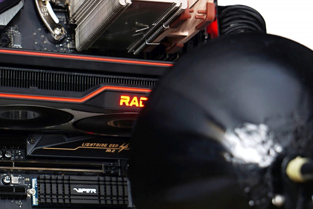
Of course, the key is to filter out all spurious frequencies that do not relate to the device being measured (such as a graphics card), so this requires passive operation of other components, while the results may be distorted by whistling coils on the motherboard or the power supply. However, we managed to eliminate all this. We will also state the intensity of the dominant frequencies. Again, in three bandwidths of low (20–200 Hz), mid (201–2,000 Hz) and high (2,001–20,000 Hz) tones. The last test of graphics cards already includes this methodology and new results will snowball with each new test.
| Graphics card | Dominant sound freq. and noise level in SOTTR@2160p | NF-F12 PWM | NF-A15 PWM | ||||
| Low range | Mid range | High range | |||||
| Frequency [Hz] | Noise level [dBu] | Frequency [Hz] | Noise level [dBu] | Frequency [Hz] | Noise level [dBu] | ||
| AMD Radeon RX 6800 XT | Ložisko | 100,794 | -73,170 | 1107,887 | -75,262 | 10848,902 | -75,397 |
| Asus TUF RTX 3080 O10G Gaming | Výška (bez ventilátoru) | 100,794 | -75,410 | 1076,347 | -72,321 | 7240,773 | -74,199 |
| AMD Radeon RX 6800 | 100,794 | -71,603 | 1140,350 | -67,765 | 9665,273 | -80,642 |
Maybe you are interested in one more thing that has not been said in the text so far. Namely, at which point we read the values that are inserted into the tables. Of course, the noise level of graphics cards changes over time according to the load. Therefore, the measured values are based on the average of the last 100 samples, which have a more or less stable form. We always read this data just before the end of the test scenes in games F1 2020, Shadow of the Tomb Raider, CS:GO and apps Blender (Cycles), Classroom. Then the fan speed is already stable and no longer increases.
So ladies and gentlemen, don’t believe in one value measured by a sound level meter so much. It’s enough for a rough orientation and an idea of how noisy a particular component is, but you will have to study its frequency analysis for accurate sound. However, you will receive all the materials for studying these properties from us. Even in the tests of coolers and measurement of the frequency response of sound, you will of course soon find in in the fan tests, which we can no longer wait for ourselves and we believe that you feel the same way.
I apologize for the potential inaccuracy of expression and incorrect terminology or imperfect technical implementation of some aspects to all sound engineers and people more erudite in acoustics than I am (I certainly do not consider myself a sound master 🙂 ). The aim of this all was to achieve the highest possible sound distinction and satisfactory repeatability of measurements with the least possible error. In addition, it was all aimed at ensuring that the results were of relevant quality, which was successful.